Top 60+ Data Science Interview Questions and Answers

Correlation is the statistical measure that shows a relationship between two variables. When one changes, the other changes as well, positively or negatively. However, this doesn't mean that one variable causes the other to change. Causation means that one variable directly causes a change in the other. It implies a cause-and-effect relationship, not just an association. Proving causation requires deeper analysis and additional evidence.

Example: There's a correlation between cart abandonment and uninstall rates in a shopping app. Users who abandon their carts often end up uninstalling the app shortly after. But that doesn't mean abandoning a cart causes someone to uninstall the app. The real cause might be a frustrating purchase process with too many steps. That complexity leads to both behaviors: abandoning the cart and uninstalling the app. So, while there's a correlation, you can't say it's causation without looking deeper.

The role of statistics in data science is to help data scientists understand and summarize data, uncover patterns, validate models, handle uncertainty (like missing or noisy data), and make evidence-based decisions.

For example:

• Mean and median summarize central tendencies.
• Standard deviation and variance measure variability.
• Hypothesis testing validates assumptions.
• Regression analysis predicts relationships between variables.
• Bayesian inference updates beliefs as new data comes in.

Use case: A marketing team runs an A/B test to compare two email campaigns. Statistical methods help determine whether the difference in click-through rates is real or just a coincidence.

After observing that my data set has missing values, I'll figure out how it occurs. Are they represented as NaN, None, empty strings, weird characters like -999, a combination of two or more, or something else?

Once I make sense of what my missing data looks like, I dig into why these values are missing, and they usually fall into three categories:

• Missing Completely At Random (MCAR): No pattern, just random gaps. These are usually safe to drop, especially if there aren't many.

  Example: In a survey dataset, 10% of income entries are missing due to a technical glitch that affected a random subset of responses. There's no pattern based on age, education, employment status, or anything else.

• Missing At Random (MAR): This is when the missing data is related to other observed variables, but not to the income value itself.

  Example: In the same dataset, 10% of income values are missing, mostly among respondents who are students. Here, missing data is related to the occupation variable, not the actual income value. Impute based on related features like occupation, education level, or age. Impute based on related features like occupation, education level, or age. Safe to drop or impute with mean/median since the missing data doesn't introduce bias.

• MNAR (Missing Not At Random): The reason it's missing is tied to the value itself.

  Example: If high spenders choose not to share income, that's tougher to handle and sometimes better tracked with a missingness flag. The probability of missingness increases with the income amount. Imputation is risky here. I'll consider flagging missingness with a binary indicator (income_missing) or using models that can account for MNAR, like EM algorithms or data augmentation techniques.

Once I know the type of missingness, I choose one of the following: a. Deletion (if safe):

• Listwise: Drop rows with missing values (only when missingness is random and small).
• Pairwise: Use available values for calculations, such as correlations.
• Drop columns: Remove low-value features with lots of missing data.

b. Simple imputation:

• Mean/Median/Mode: Use for numeric or categorical columns, depending on distribution.
• Arbitrary values: Fill with 0 or "Unknown" if it makes sense contextually.
• Forward/Backward fill: Best for time series to keep temporal consistency.

c. Advanced imputation:

• KNN imputer: Fills gaps by finding similar rows using distance metrics.
• Iterative imputer: Builds a model with other columns to estimate missing values.
• Interpolation: Good for numeric sequences, especially when data follows a trend.

d. Use missingness as a feature:

• If the missing value could carry a signal, I add a binary indicator column (e.g., was_missing = 1).

e. Oversampling or undersampling:

• If missing data causes class imbalance, I use resampling to maintain a fair target distribution.

Common pitfall: Filling in values without understanding the pattern of missingness. For example, using mean imputation on MNAR data can introduce bias and weaken your model's predictive power.

Univariate analysis is all about looking at one variable on its own, with no comparisons, just understanding its distribution, central tendency, or spread. For example, I might look at the average test score in a class or the frequency of different grade ranges using histograms or summary statistics.

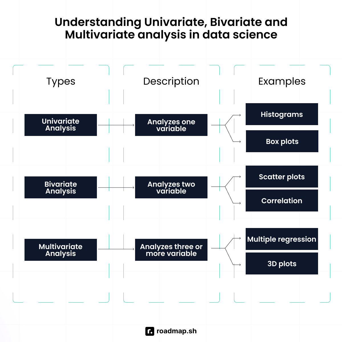
Bivariate analysis looks at the relationship between two variables, such as how students' study time affects their test scores. To analyze this, I'd use tools like correlation, scatter plots, or line graphs to identify trends or patterns.

Multivariate analysis, on the other hand, deals with three or more variables at once. It focuses on understanding how multiple factors combine to influence an outcome. For example, I might explore how sleep hours, study time, and caffeine intake together impact test scores. In that case, I'd use regression or a tree-based model to analyze the combined effect.

The difference between long format data and wide format data comes down to how your data is structured. A wide format has values that do not repeat in the columns, while a long format has values that do repeat in the columns.

In wide format, you spread data across columns. Each variable (Jan, Feb, March) gets its own column. You'll usually see this in reports or dashboards.

In long format, data is stacked in rows. One column stores the values, and another column tells you what those values represent. This format is cleaner for grouped summaries and time series analysis.

Use case: Wide format is useful for reporting and making data visualizations. Long format is preferred for time series, grouped summaries, and plotting tools like Seaborn or ggplot.

Common pitfall: Trying to perform group-level analysis on wide-format data without reshaping it first.

Multicollinearity is when two or more independent variables in a regression model are highly correlated, meaning they tell similar stories. This makes it hard for the model to figure out which variable is actually influencing the target, leading to unreliable or unstable coefficient estimates.

For example, in a regression model looking at economic growth, common variables will be GDP, Unemployment Rate, and Consumer Spending. These variables are all related, and the model might not be as effective as it should be.

To detect multicollinearity use:

• Correlation matrix: A correlation matrix detects multicollinearity by visualizing the strength of relationships between variables. A general rule is that any correlation value above 0.6 indicates strong multicollinearity.
• Variance inflation factor (VIF): VIF detects multicollinearity by giving a numerical value that indicates how much the variance of a regression coefficient is inflated due to multicollinearity. A VIF value greater than 5 indicates moderate multicollinearity, while values above 10 suggest severe multicollinearity.
• Condition index: The condition index is a tool for detecting multicollinearity. Values above 10 indicate moderate multicollinearity, and values above 30 indicate severe multicollinearity. The condition index works by checking how much the independent variables are related to each other by examining the relationships between their eigenvalues.

Common pitfall: Including highly correlated predictors without checking VIF may inflate model error and reduce stability.

Variance in data science measures the spread between numbers in a dataset. Simply put, it measures how far each number in the set is from the mean (average). It helps us understand how spread out or consistent the values are in a dataset.

Low variance example: Mean: (78 + 79 + 80 + 81 + 82) / 5 = 80

Imbalanced data is a situation where the classes, labels, or categories in a dataset are not equally represented. In imbalanced datasets, one category has significantly more or fewer samples than the others. Imbalanced data refers to a common issue in supervised machine learning and deep learning where there is a non-uniform distribution of samples among different classes. This can lead to biased outcomes in models, such as those used in healthcare services, impacting their reliability and effectiveness.

For example, if you build an email spam detection model and your dataset contains 5% spam emails and 95% non-spam emails, the data is imbalanced toward non-spam. This imbalance can negatively affect the model's performance, especially in production, because it may achieve high accuracy by simply predicting the majority class while failing to detect spam effectively.

A categorical variable is a column with fixed options based on qualities or labels like gender, age group, or education level. You can't do math on them directly, so during preprocessing, I usually apply one-hot encoding to turn those categories into binary columns the model can understand.

A continuous variable, on the other hand, can take on any value within a range like height, temperature, or speed. These are numeric, so you can run calculations on them. But before feeding them into a model, I scale them using normalization or standardization to keep all features on a similar range. This prevents one feature from overpowering the rest just because it has larger numbers.

To transform data from wide format to long format, I usually use the melt() function in pandas to unpivot the columns into rows. It's especially useful when you have repeated measures across columns, like monthly sales or survey responses, and you want to make the data tidy for analysis or plotting.

For example, if I have a DataFrame where each column represents a month, I'll keep the identifier (like product name) as is, and melt the rest so each row shows one product-month-sales combo. This makes it easier to group, filter, or feed into models.

When I combine data from different sources with inconsistent formats, the first thing I do is standardize everything: dates, column names, booleans, numbers, etc., so they all speak the same language. After doing that, I'll:

• Align schemas: match columns across datasets. If one has extras, I drop or keep them depending on relevance.
• Unify categories: I clean up inconsistencies like "Y" vs. "Yes" to avoid downstream issues.
• Tag the source: I add a source column so I know where each row came from. This is super useful for tracking or debugging later.
• Merge or stack: If the structure is the same, I concat(). If I'm matching on something like customer ID, I go with a merge or join.
• Final clean-up: I look for duplicates, mismatched types, or broken values post-merge and fix them.

I avoid merging before checking data types or keys. That’s a fast track to lost or duplicated rows.

The Central Limit Theorem (CLT) states that if you take enough random samples from any dataset, even if the data is skewed or messy, the average of those samples will start to form a bell-shaped or normal distribution. This only holds if the samples are random, independent, and large enough, usually 30 or more.

Why does this matter? Because once those averages form a normal shape, you can use all the tools from the normal distribution. You can calculate standard errors, build confidence intervals, run hypothesis tests, make estimates, and use z-scores, even if the original data wasn’t normal to begin with.

The difference between Type I and Type II error is that Type I error rejects a true null hypothesis (a false positive), while Type II error fails to reject a false null hypothesis (a false negative).

Let's assume you're testing a new drug. The null hypothesis is that the drug doesn't work, and in reality, it indeed doesn't. A type I error occurs when your test says it does, but it doesn't; this is a false positive. A type II, on the other hand, is when the drug works in reality, but your tests say it doesn't: a false negative.

A p-value is a statistical measure that determines the significance of the result you got in a hypothesis test. A small p-value (<0.05) indicates strong evidence that the null hypothesis is wrong, meaning you should reject it.

If the probability of the p-value is greater than 0.05, there is not enough evidence to reject the null hypothesis. For example, if you conduct an experiment and the p-value is 0.03, you should reject the null hypothesis.

A confidence interval is a range of values that's likely to have the true value of a population parameter based on sample data. Let's say you surveyed a sample of high school teachers and found their average salary was $75,000. Since that's just a sample, you can't say for sure it reflects all teachers, but we can say:

"We're 95% confident that the real average salary for all teachers falls between $72,000 and $78,000."

The confidence interval is between $72,000 and $78,000. It gives us a buffer to account for uncertainty in our estimate.

A probability distribution tells you how likely different possible outcomes are for a random event or experiment. It maps out the chances of different results happening. It’s a way of saying, “Here’s everything that could happen, and how often I expect each one to happen.”

The commonly used probability distributions are normal (bell curve), binomial, Poisson, and uniform distributions.

Common pitfall: Different types of distributions need different types of analysis. Using the wrong type of distribution for analysis can lead to wrong results. Another common problem is assuming that data follow a normal distribution without testing for normality.

The difference between a t-test and a z-test comes down to what you know about your data: the sample size and the population standard deviation.

Use a t-test when:

• The sample size is small (usually n ≤ 30).
• The population standard deviation is unknown.
• You still want to compare means (sample vs. population or between two samples).

Use a z-test when:

• You know the population standard deviation.
• Your sample size is large (typically n > 30).
• The data is roughly normally distributed.

The null hypothesis (H₀) is the starting point and default assumption of every statistical analysis. The idea is that there's nothing happening in your data: no stories, no effect, no relationship between the variables you're testing until your data gives strong evidence to reject it.

To know whether to reject the null hypothesis, here's what I do:

First, I set a significance level, usually 0.05. Then, I calculate the p-value. If the p-value is less than or equal to 0.05, I reject the null hypothesis because the result is statistically significant. If it's more than 0.05, I don't reject it because there isn't enough evidence.

This is a curveball question because the interviewer isn't really asking about the classic CLT. They're testing your knowledge about the Lindeberg-Feller CLT.

In the classic CLT, all the variables are independent and from the same probability distribution (identically distributed). But here, the interviewer is saying: What if they're still independent but not identically distributed? Lindeberg-Feller helps in situations like this.

It states that as long as the variables are independent, have finite second moments (meaning their variances aren't huge), and no single variable dominates (the Lindeberg condition), the normalized sum of those variables will still approach a normal distribution. So, even with different distributions, if those conditions hold, the average still forms a bell curve.

A long-tail distribution is a type of distribution where you group most of the data around the middle, but there are still many rare or unusual values that stretch far out to the sides (tail) and have a big impact.

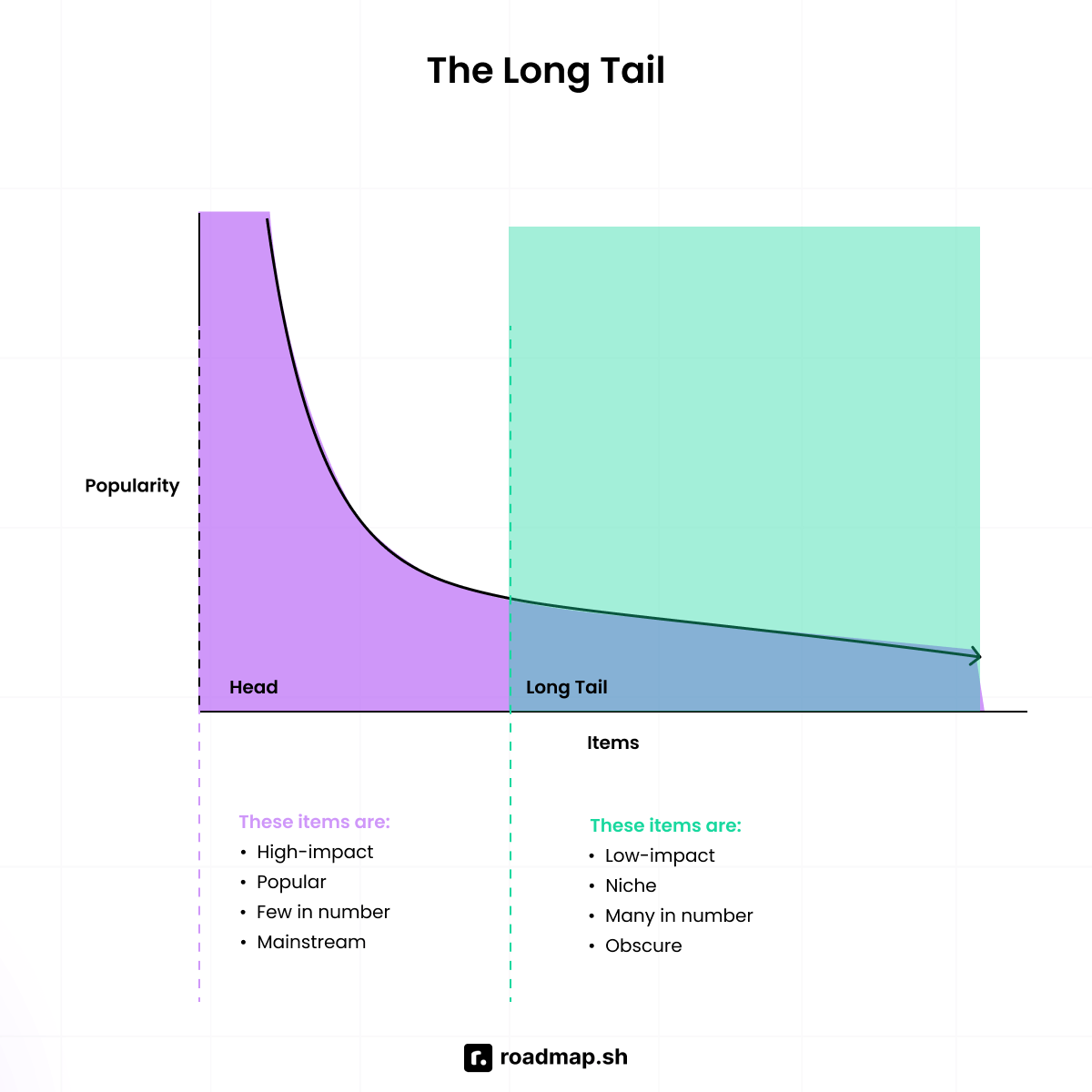
Some examples are:

1. Long-tail keywords in SEO: A few high-volume keywords (like "shoes") get massive search volume, but there's a long tail of specific, niche searches (like "waterproof hiking shoes for wide feet") that collectively make up most of the search traffic. These long-tail keywords aren't often searched for, but they convert well.

2. Book sales: Bestsellers like Harry Potter dominate the market, but tons of niche books (even classics like Jane Austen) sell steadily in the background. The collective sales of these less popular books often exceed those of the bestsellers.

3. Luxury bags: A few brands are always trending. However, there's a long list of unique, lesser-known ones that still sell and matter to the market.

Why they're important in classification and regression problems:

Long-tail distributions can throw off model performance because most models are trained on the majority class, the "head," and ignore rare but important events in the tail. This is risky in cases like fraud detection or churn modeling, where rare events matter most. They also affect Mean Squared Error, which squares the difference between predicted and actual values, so a few extreme errors from tail cases can blow up the score, even if your model does well overall.

Long-tail distributions can create models that are biased toward the majority, skew errors, and cause you to miss rare events that matter. Handling them requires better sampling techniques and using loss functions that properly account for these rare but significant occurrences.

The difference between supervised, unsupervised, and reinforcement learning lies in how the model learns. This table describes their contrasts and common use cases for each.

The bias-variance tradeoff refers to the balance between a model's ability to learn patterns (low bias) and its ability to generalize to new data (low variance). Bias is the error made when the model makes strong assumptions about the data: high bias could lead to underfitting. Variance is the model's sensitivity to small fluctuations in the data, and high variance could lead to overfitting.

Cross-validation is a technique for evaluating a model's performance on an individual dataset. It divides the dataset into subsets, usually the training, test, and validation sets. This process is repeated multiple times to ensure the model generalizes well to unseen data and to stop overfitting.

Overfitting in machine learning happens when the model learns from the training data too well, including non-relevant details. This leads the model to perform very well on the training data but poorly on other data.

Prevention techniques:

• Regularization (L1/L2): This method adds a penalty to large weights to keep the model from becoming too complex.
• Cross-validation: This helps test the model on different slices of data to make sure it generalizes well.
• Pruning (for tree models): Cuts back unnecessary branches that overcomplicate the model.
• Early stopping: Stops training when performance stops improving on the validation set.
• Dropout (for neural nets): This method randomly drops neurons during training so the network doesn't become too dependent on specific paths.

A decision tree is a machine learning algorithm used for classification and regression tasks. It makes decisions by following a tree-like structure where internal nodes represent attribute tests, branches represent attribute values, and leaf nodes represent predictions.

Decision trees are versatile and are used for many machine learning tasks.

Example: Loan approval decision tree

• Step 1 – Ask a question (Root Node): Is the applicant's credit score > 700?
  • If yes, go to Internal Node.
  • If no, go to Leaf Node (Do not approve the loan).
• Step 2 – More questions (Internal Nodes): Is the applicant's income > $50,000?
  • If yes, approve the loan (Leaf Node).
  • If no, go to Leaf Node (Do not approve the loan).
• Step 3 - Decision (Leaf Node)
  • Leaf Node 1: Do not approve the loan (if credit score ≤ 700).
  • Leaf Node 2: Approve the loan (if credit score > 700 and income > $50,000).
  • Leaf Node 3: Do not approve the loan (if credit score > 700 and income ≤ $50,000).

Common pitfall: Trees tend to overfit the data if you allow it to go too deep and include too many branches.

This table describes the difference between decision trees and random forests and when to use them based on features like accuracy, training time, etc.

A random forest is a collection of multiple decision trees, while a decision tree is just a single model that predicts outcomes based on a series of decisions. For a random forest, each tree is trained on a subset of the data and a subset of features, and both of these are random. A decision tree is a simple, tree-like structure used to represent decisions and the possible outcomes from them. Random forest multiple trees use bootstrapped samples and random feature selection, then average predictions to improve accuracy and reduce overfitting.

Logistic regression is a supervised machine learning algorithm commonly used for binary classification tasks by predicting the probability of an outcome, event, or observation. The model delivers a binary outcome limited to two possible outcomes: yes/no, 0/1, or true/false. Logical regression analyzes the relationship between one or more independent variables and classifies the data into discrete classes. This relationship is then used to predict the value of one of those factors, the probability of a binary outcome using the logistic (sigmoid) function. It is mostly used for predictive modeling.

For example, 0 represents a negative class, and 1 represents a positive class. Logistic regression is commonly used in binary classification problems where the outcome variable reveals either of the two categories (0 and 1).

Common pitfall: Misunderstanding that logistic regression is not a classification algorithm but a probability estimator.

Linear regression is a statistical method used to model the relationship between a dependent variable and one or more independent variables. It is a type of supervised machine learning algorithm that computes the linear relationship between the dependent variable and one or more independent features by fitting a linear equation with observed data. It predicts the output variables based on the independent input variable.

For example, if you want to predict someone's salary, you use various factors such as years of experience, education level, industry of employment, and location of the job. Linear regression uses all these parameters to predict the salary as it is considered a linear relation between all these factors and the price of the house.

Assumptions for linear regression include:

• Linearity: Linear regression assumes there is a linear relationship between the independent and dependent variables. This means that changes in the independent variable lead to proportional changes in the dependent variable, whether positively or negatively.
• Independence of errors: The observations should be independent from each other, that is, the errors from one observation should not influence another.
• Homoscedasticity (equal variance): Linear regression assumes the variance of the errors is constant across all levels of the independent variable(s). This indicates that the amount of the independent variable(s) has no impact on the variance of the errors.
• Normality of residuals: This means that the residuals should follow a bell-shaped curve. If the residuals are not normally distributed, then linear regression will not be an accurate model.
• No multicollinearity: Linear regression assumes there is no correlation between the independent variables chosen for the model.

A Support Vector Machine (SVM) is a supervised machine learning algorithm used mainly for classification tasks. It finds the optimal hyperplane in an N-dimensional space that separates data points into different classes while maximizing the margin between the closest points of each class.

Support vectors are the most important data points, useful in defining the optimal hyperplane that separates different classes.

KNN stands for K-nearest neighbors is a classification (or regression) algorithm that, to determine the classification of a point, combines the classification of the K nearest points. It is supervised because you are trying to classify a point based on the known classification of other points.

K-means is a clustering algorithm that tries to partition a set of points into K sets (clusters) such that the points in each cluster tend to be near each other. It is unsupervised because the points have no external classification.

This table shows the difference between KNN and K-means depending on the use case, data usage, purpose, and other features.

Ensemble techniques in machine learning combine multiple weak models into a strong, more accurate predictive model, using the collective intelligence of diverse models to improve performance. Bagging and boosting are different ensemble techniques that use multiple models to reduce error and optimize the model.

The bagging technique uses multiple models trained on different subsets of data. It decreases the variance and helps to avoid overfitting. It is usually applied to decision tree methods and is a special case of the model averaging approach. Boosting is an ensemble modeling technique designed to create a strong classifier by combining multiple weak classifiers. The process involves building models sequentially, where each new model aims to correct the errors made by the previous ones.

• Bagging: Builds multiple models in parallel using bootstrapped datasets to reduce variance (e.g., Random Forest).
• Boosting: Builds models sequentially, each trying to correct errors from the previous, reducing bias (e.g., XGBoost).

A linear regression algorithm defines a linear relationship between independent and dependent variables. It uses a linear equation to identify the line of best fit (straight line) for a problem, which it then uses to predict the output of the dependent variables.

A logistic regression algorithm predicts a binary outcome for an event based on a dataset's previous observations. Its output lies between 0 and 1. The algorithm uses independent variables to predict the occurrence or failure of specific events.

You use linear regression when the outcome is a continuous value, such as price or temperature. You should use logistic regression when the outcome is a categorical value like spam/not spam, yes/no, etc.

Regularization is a technique in machine learning to prevent models from overfitting. Overfitting happens when a model doesn't just learn from the underlying patterns (signals) in the training data but also picks up and amplifies the noise in it. This leads to a model that performs well on training data but poorly on new data.

L1 and L2 regularization are methods used to mitigate overfitting in machine learning models by adding a penalty term on coefficients to the model's loss function. This penalty discourages the model from assigning too much importance to any single feature (represented by large coefficients), making the model more straightforward. Regularization keeps the model balanced and focused on the true signal, enhancing its ability to generalize to unseen data.

A regression model that uses the L1 regularization technique is called lasso regression, and a model that uses the L2 is called ridge regression.

• L1 Regularization: Also called a lasso regression, this adds the absolute value of the sum ("absolute value of magnitude") of coefficients as a penalty term to the loss function.
• L2 Regularization: Also called a ridge regression, this adds the squared sum ("squared magnitude") of coefficients as the penalty term to the loss function.

Once a machine learning model has been created, it is important to evaluate and test how well it performs on data. An evaluation metric is a mathematical quantifier of the quality of the model. Precision, Recall, F1 Score, and AUC-ROC are all evaluation metrics.

• Precision is all about how accurate your positive predictions are. Of all the items your model labeled as positive, how many were actually positive? Formula = TP / (TP + FP). It tells you how much you can trust the positives your model finds.
• Recall focuses on finding all the actual positives. It measures how well your model catches everything it should've caught. Formula = TP / (TP + FN). It's especially useful when missing a positive is costly like missing a cancer diagnosis.
• F1 Score: F1 Score combines Recall and Precision into one performance metric. The F1 Score is the weighted average of Precision and Recall. Therefore, this score takes both false positives and false negatives into account. F1 is usually more useful than Accuracy, especially if you have an uneven class distribution.
• AUC-ROC: The AUC-ROC curve is a tool for evaluating the performance of binary classification models. It plots the True Positive Rate (TPR) against the False Positive Rate (FPR) at different thresholds, showing how well a model can distinguish between two classes, such as positive and negative outcomes. It provides a graphical representation of the model's ability to distinguish between two classes, like a positive class for the presence of a disease and a negative class for the absence of a disease.

Key: TP = True Positive, FP = False Positive, FN = False Negative.

A confusion matrix is a simple table that shows how well a classification model is performing by comparing its predictions to the actual results. It breaks down the predictions into four categories: correct predictions for both classes (true positives and true negatives) and incorrect predictions (false positives and false negatives). This helps you understand where the model is making mistakes so you can improve it.

• TP: True Positives
• TN: True Negatives
• FP: False Positives
• FN: False Negatives

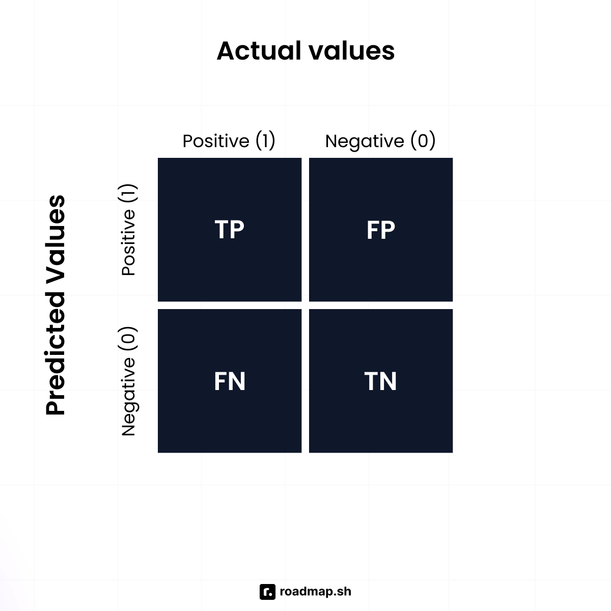
Example: From the matrix below, there are 165 total cases:

• True Negatives: 50
• False Positives: 10
• False Negatives: 5
• True Positives: 100

Depending on the project you're working on, you can use metrics such as Accuracy, Precision, Recall, and F1 Score to evaluate your project. A confusion matrix is a visualization of it.

Common pitfall: Misreading the matrix layout or assuming it works for multi-class without modification.

When building a predictive model, I like to combine practical steps and proven techniques to ensure that the features I include actually help the model rather than add noise, redundancy, or overfitting risk.

I'll approach like this:

1. Start with domain knowledge: Talk to stakeholders and review documentation to understand what features make the most sense in our business context.
2. Use filter methods for a first pass: I run statistical checks like correlation, ANOVA, chi-square tests, or mutual information to remove irrelevant or redundant features. Filter methods are fast, which is especially helpful when you're working with high-dimensional data.
3. Apply wrapper methods for performance tuning: For a more refined selection, I use wrapper methods like Recursive Feature Elimination (RFE). These methods evaluate subsets of features based on how well the model performs, which helps surface the most predictive combinations. They take more time but are worth it for high-impact models.
4. Leverage embedded methods for efficiency: Models like Lasso (L1), Ridge (L2), and tree-based models (Random Forest, XGBoost) have built-in feature importance. I like these because they optimize feature selection during model training, balancing speed and accuracy.
5. Hybrid approach: Sometimes, I start with a filter method to reduce dimensions and then fine-tune with wrapper or embedded methods. This hybrid approach saves time and improves performance.

How I decide what to drop or keep:

• If a feature is highly correlated with another, I drop the weaker or noisier one.
• If it has low variance and no predictive power, it goes.
• If it helps interpretability or improves metrics on validation data, I keep it.
• If it harms generalization or adds complexity, I drop it.

False Positive Rate (FPR) is the proportion of actual negatives that are incorrectly identified to be true. False Negative Rate is the proportion of actual positives that are incorrectly identified as negatives.

In a fraud detection scenario, both of these have damaging consequences:

False Positive Rate (FPR): If a model has a high false positive rate, it means the system flags many legitimate transactions as fraudulent. This will lead to customer frustration, as their transactions will be flagged regularly, and they could leave.

False Negative Rate (FNR): If a model has a high false negative rate, it means many fraudulent transactions are not detected, which could lead to significant financial business loss.

To find the second highest salary, you can take one of two common methods: a subquery or a window function.

Method 1: Subquery method You first get the maximum salary from the table. Then, you find the highest salary that's less than that max, giving you the second highest salary.

This method is clean and efficient:

SELECT MAX(salary) AS SecondHighest
FROM employee
WHERE salary < (SELECT MAX(salary) FROM employee);

Method 2: Window function with DENSE_RANK() You rank all salaries in descending order using DENSE_RANK(), then filter for rank 2 to get the second highest. The LIMIT 1 ensures only one row is returned in case of ties. This method is better for flexibility if you want to choose the third highest or fourth, etc.

SELECT salary AS SecondHighest
FROM (
  SELECT salary, DENSE_RANK() OVER (ORDER BY salary DESC) as rank
  FROM employee
) ranked
WHERE rank = 2
LIMIT 1;

To join order details with corresponding customer information, you use a simple inner join:

SELECT o.*, c.name, c.email
FROM orders o
JOIN customers c ON o.customer_id = c.id;

This pulls all orders where a matching customer exists. If you need every order, even those without matching customers, switch to a LEFT JOIN:

SELECT o.*, c.name, c.email
FROM orders o
LEFT JOIN customers c ON o.customer_id = c.id;

To get the highest-spending customers, group by customer, sum their order totals, sort by that total, and limit the results:

SELECT customer_id, SUM(total_amount) AS revenue
FROM orders
GROUP BY customer_id
ORDER BY revenue DESC
LIMIT 5;

To add customer names, just join with the customers' table.

Common pitfall: Not grouping properly before ordering can result in incorrect aggregates.

To find your top customers who also bought across multiple categories, filter purchases within 3 months, group by customer, and apply category constraints with HAVING:

SELECT customer_id, SUM(amount) AS total_spent
FROM purchases
WHERE purchase_date >= DATE_SUB(CURDATE(), INTERVAL 3 MONTH)
GROUP BY customer_id
HAVING COUNT(DISTINCT category_id) >= 3
ORDER BY total_spent DESC
LIMIT 5;

This makes sure each customer bought from at least 3 categories. WHERE filters rows before grouping, while HAVING filters groups after.

To remove duplicates from a DataFrame:

df = df.drop_duplicates()

You can also refine this by specifying columns:

# Drop duplicates based on specific columns
df = df.drop_duplicates(subset=['customer_id', 'product_id'])

Control which duplicates to keep:

# Keep first or last occurrence
df = df.drop_duplicates(keep='last')  # or 'first'

To compute the median in a stream of numbers, use two heaps:

• Max-heap for the lower half
• Min-heap for the upper half
• Keep both heaps balanced
• The median is either the top of one heap or the average of both tops

import heapq

class MedianFinder:
    def __init__(self):
        self.small = []  # max heap (negative values)
        self.large = []  # min heap
    
    def add_num(self, num):
        if len(self.small) == len(self.large):
            heapq.heappush(self.large, -heapq.heappushpop(self.small, -num))
        else:
            heapq.heappush(self.small, -heapq.heappushpop(self.large, num))
    
    def find_median(self):
        if len(self.small) == len(self.large):
            return (self.large[0] - self.small[0]) / 2.0
        else:
            return self.large[0]

To merge overlapping intervals, first sort them, then iterate and merge as needed:

def merge_intervals(intervals):
    intervals.sort(key=lambda x: x[0])
    merged = [intervals[0]]
    for current in intervals[1:]:
        last = merged[-1]
        if current[0] <= last[1]:
            last[1] = max(last[1], current[1])
        else:
            merged.append(current)
    return merged

Sorting takes O(n log n), and the merge step is linear, making this efficient for large datasets.

Basic null handling options:

df.fillna(0)      # Replace with 0  
df.dropna()       # Drop rows with nulls

Other methods to consider:

# Fill with mean/median/mode
df['column'].fillna(df['column'].mean())
df['column'].fillna(df['column'].median())
df['column'].fillna(df['column'].mode()[0])

# Forward/backward fill
df.fillna(method='ffill')  # Use previous value
df.fillna(method='bfill')  # Use next value

# Interpolation
df.interpolate()

Basic group and sum:

df.groupby('category')['sales'].sum()

For more complex aggregations:

# Multiple aggregations
df.groupby('category').agg({
    'sales': ['sum', 'mean', 'count'],
    'profit': ['min', 'max']
})

# Custom aggregation functions
df.groupby('category')['sales'].agg(lambda x: x.max() - x.min())

# Reset index to convert back to a regular DataFrame
df.groupby('category')['sales'].sum().reset_index()

Given values: 100, 90, 90, 80
RANK(): Skips ranks after ties
→ 1, 2, 2, 4
DENSE_RANK(): No skipping
→ 1, 2, 2, 3
ROW_NUMBER(): Ignores ties
→ 1, 2, 3, 4

A RIGHT JOIN is the same as a LEFT JOIN with the table order reversed:

SELECT * FROM A RIGHT JOIN B ON A.id = B.id;
SELECT * FROM B LEFT JOIN A ON A.id = B.id;

• .map(): Works only on Series, applies a function element-wise
• .apply(): More versatile, works on both Series and DataFrames
• .applymap(): Applies a function to every element in a DataFrame

# map - simple transformation of Series values
df['category'] = df['category_id'].map({1: 'Electronics', 2: 'Clothing'})

# apply on Series - more complex operations
df['name'] = df['name'].apply(lambda x: x.title())

# apply on DataFrame - process entire rows or columns
df.apply(lambda x: x.max() - x.min())

# applymap - element-wise operation on entire DataFrame
df.applymap(lambda x: f"{x:.2f}" if isinstance(x, float) else x)

Basic usage:

from sklearn.cluster import KMeans  
kmeans = KMeans(n_clusters=3).fit(X)
labels = kmeans.labels_

Best practices for K-Means:

# Scale features
from sklearn.preprocessing import StandardScaler
X_scaled = StandardScaler().fit_transform(X)

# Use elbow method to find optimal k
distortions = []
K_range = range(1, 10)
for k in K_range:
    kmeans = KMeans(n_clusters=k, random_state=42)
    kmeans.fit(X_scaled)
    distortions.append(kmeans.inertia_)

# Plot elbow curve
import matplotlib.pyplot as plt
plt.plot(K_range, distortions)
plt.xlabel('k')
plt.ylabel('Distortion')
plt.title('Elbow Method For Optimal k')

To evaluate a regression model:

from sklearn.metrics import mean_squared_error  
import numpy as np  
mse = mean_squared_error(y_true, y_pred)  
rmse = np.sqrt(mse)

• MSE: Penalizes large errors heavily.
• RMSE: More interpretable because it's in the same unit as the target.

Another alternative:

from sklearn.metrics import mean_absolute_error
mae = mean_absolute_error(y_true, y_pred)

MAE is less sensitive to outliers.

accuracy = (TP + TN) / (TP + TN + FP + FN)
precision = TP / (TP + FP)  # How many selected items are relevant
recall = TP / (TP + FN)     # How many relevant items are selected
f1_score = 2 * (precision * recall) / (precision + recall)  # Harmonic mean

# For imbalanced datasets, consider:
specificity = TN / (TN + FP)
balanced_accuracy = (recall + specificity) / 2

First, define success for that specific launch. Is it getting 1,000 new users in 30 days? Hitting a revenue or CTR goal? Building awareness in a new market? Or collecting feedback for future improvements?

Once that's clear, measure success using a mix of quantitative and qualitative KPIs across teams like marketing, product, and customer success. Some metrics I'll look at:

• Launch campaign metrics: To gauge marketing performance, look at leads generated, channel performance (email, ads, social), website traffic, and press coverage.
• Product adoption metrics: After launch, track trials, usage, activation, and user retention. These show how well the product is landing with your target audience.
• Market impact metrics: Measure business impact through revenue, market share, and win rates against competitors.
• Qualitative feedback: Talk to sales reps, product teams, and customers. Internal and external feedback helps you understand the "why" behind the numbers. Blending data with direct feedback gives you a more transparent, more nuanced view of what's working and what to improve.

Common pitfall: Focusing only on quantitative metrics without applying nuance to them. An example is tracking metrics like downloads without tracking engagement. Or tracking views without knowing who is viewing them.

To analyze a sudden drop in website traffic, I would follow these steps:

• Determine if it's a drop or a trend: The first thing to do is try to understand whether your traffic has been declining for a while or if it has suddenly dropped for a day or two.
• Rule out any manual actions: Sometimes, traffic drops happen because of a Google penalty. Check to see if there are any recent changes that you might have fallen foul of. Also, make sure that updates you made to your website's content didn't cause a problem.
• Check for algorithm updates: Google frequently updates its ranking algorithm. When your site's performance drops suddenly, it's worth investigating whether an update might be responsible.
• Investigate technical issues: Some of the most common technical issues are indexing errors, site speed, performance, and mobile usability.
• Check competitor activity: Sometimes, traffic dips occur because competitors have stepped up their game. SEO tools like Ahrefs, SEMrush, or Moz help track your competitors' backlinks, keywords, and rankings. Check to see whether your competitors have started outranking you for previously held keywords or launched new content targeting your primary audience.

There could be multiple reasons why a business could be unsatisfied with a model that has high accuracy. Some reasons are:

• Focusing on the wrong metric: Sometimes, a model is not optimized for the specific business problem. Its accuracy is tied to the wrong thing. For example, in fraud detection, it is possible to still miss fraudulent transactions even with high accuracy scores.
• Unrealistic expectations: The model might have unrealistic expectations placed on it to solve problems when, in reality, it is meant to be used in conjunction with other methods and metrics to give a nuanced view.
• Overfitting: It is possible that the high accuracy comes from the model learning the training data rather than learning how to generalize.

To handle this problem, I'll:

• Reevaluate the business goals: Sometimes, the business goals need to be defined so that there is a specific metric or group of metrics for the model to be trained towards.
• Improve the model performance: You should do a deep dive into the model and fix any issues that you might notice, including overfitting, data issues or feature selection.

To check the quality of a random dataset, I'll:

• Understand the problem context: The first thing to do is to make sure you understand the goal you aim to achieve before looking at the dataset. This allows you to know from first glance whether the dataset matches the problem. If the data has irrelevant columns, you should remove them.

• Test the data quality: For any problem you are solving, it has most likely been solved before. You can test your dataset against a trusted dataset to measure any deviations that might be in the data. The dataset also needs to represent real-world scenarios.

• Technical checks: With technical checks, it's good to remove duplicates in the data. Noise could be present with blurry images or mislabeled samples. You also have to make sure everything is formatted correctly in a consistent format.

• Assess practical utility: The dataset has to be big enough for what you need it to do. For traditional machine learning, the dataset should be more than 10 times greater than the number of features per class. For deep learning, you should aim for 100 features per class to help avoid overfitting.

A dataset is only useful when it aligns with the problem's context and goals. It must pass accuracy, completeness, and balance checks. Finally, it must meet size and representative requirements.

Healthcare classification models use machine learning to analyze vast amounts of patient data. They identify complex patterns and relationships, helping healthcare professionals predict health risks more accurately. These models help doctors make the right decision and reduce diagnostic errors. To evaluate classification models, you have to know the right metrics to use.

• Accuracy, sensitivity, and specificity metrics: Accuracy, sensitivity, and specificity are critical in evaluating medical models. Accuracy measures the overall correctness of predictions. Sensitivity, or recall, shows the model's ability to identify positive cases. Specificity indicates how well it identifies negative cases. These metrics are vital for diagnostic accuracy assessment in various medical fields.
• ROC curves and AUC analysis: ROC curves and AUC analysis are key metrics for healthcare AI performance. They evaluate a model's ability to distinguish between classes at different thresholds. A higher AUC score means better performance in distinguishing between positive and negative cases.
• Cross-validation techniques: Cross-validation estimates a model's performance on unseen data. Techniques like k-fold cross-validation split data into subsets for training and testing, providing a robust assessment of the model's ability to generalize.

Batch learning is a term in artificial intelligence that refers to the process of training a machine learning model on a large set of data all at once, instead of continuously updating the model as new data comes in. This method allows for greater consistency and efficiency in the training process, as the model can learn from a fixed set of data before being deployed for use.

In batch learning, the model sees the entire dataset multiple times (known as epochs), refining its understanding with each pass. By processing data in large chunks, it converges more slowly but generally achieves higher accuracy.

Online learning takes a continuous, incremental approach. Instead of waiting for all the data to be available, you feed it to the model bit by bit, just like learning something new every day instead of cramming for a final exam. The model updates with each new data point, so it's constantly learning and evolving.

For example, imagine you're monitoring customer behavior on a website. Every time a user clicks or makes a purchase, your model gets smarter, learning from that single interaction and refining its predictions for the next.

Deep learning uses multi-layered neural networks to handle complex tasks like image recognition, NLP, and recommendation systems. Think CNNs, RNNs, and Transformers.

Pros:

• Handles complex, high-dimensional data (images, audio, text)
• Works with both structured and unstructured data
• Learns non-linear relationships
• Scales well across use cases with techniques like transfer learning
• Great at generalizing from large datasets

Cons:

• Requires lots of data and compute
• Heavily dependent on data quality
• Hard to interpret (black box)
• Comes with privacy and security concerns

Traditional ML uses simpler, more interpretable algorithms like decision trees, logistic regression, and support vector machines.

Pros:

• Works well with smaller datasets
• Faster to train and more straightforward to interpret
• Lower computational cost
• More transparent and explainable

Cons:

• Struggles with complex/non-linear data
• Needs manual feature engineering
• Doesn't scale well with large datasets
• Can overfit if not tuned properly

You monitor model performance in production by tracking both functional and operational metrics.

Functional monitoring checks the health of the data and the model:

• Data quality: Monitor for missing values, duplicates, and syntax errors.
• Data/feature drift: Compare current input data to training data using stats like KL divergence, PSI, chi-squared, etc.
• Model drift: Check if model accuracy drops over time due to changing patterns in the data.

Operational monitoring keeps the system running smoothly:

• System health: Tracks latency, errors, and memory usage.
• Input data health: Watch for type mismatches, nulls, and out-of-range values.
• Model performance: Use precision/recall, RMSE, or top-k accuracy depending on the use case.
• Business KPIs: Tie model performance to actual business outcomes (e.g., conversions, revenue impact).

Concept drift happens when the relationship between your input features and target variable changes over time, causing your model's performance to drop. It's common in dynamic environments (e.g., user behavior, market trends). COVID-19 is a real-world example: models trained pre-pandemic broke down because behavior and data patterns shifted.

How to detect it:

• Set up reference vs. detection windows: Compare a stable past dataset (e.g., January traffic) against a current window (e.g., this week). This gives you a baseline.
• Compare distributions: Use statistical tests (e.g., Kolmogorov–Smirnov, PSI, KL divergence) to detect shifts in data or feature distributions.
• Track model performance over time: Drop in precision, recall, or overall accuracy compared to your baseline = red flag.
• Run significance tests: This tells you if the drift is real or just noise.

Fairness means your model makes decisions that don't unfairly favor or penalize any group. Bias can sneak in at any stage, like data collection, labeling, training, and even deployment, so it needs to be addressed early and often.

How to ensure fairness:

• Start with diverse training data: Your data should reflect all the groups your model impacts. If it's skewed, the model will be too.
• Preprocess to balance representation: Use techniques like oversampling underrepresented groups or reweighting the data.
• Use bias detection tools: Libraries like Fairlearn, AIF360, and What-If Tool can help you spot performance gaps across subgroups.
• Apply fairness constraints during training: Use regularization, adversarial debiasing, or post-processing adjustments to reduce harm to specific groups.
• Build transparency into the model: Use interpretable models (e.g., decision trees, linear models) or explanation tools like SHAP and LIME.
• Audit regularly across subgroups: Don't rely only on overall accuracy—look at performance across gender, race, age, etc.
• Bring in human oversight: Humans should always be part of the loop, especially in high-stakes decisions (e.g., lending, hiring).

Fine-tuning a model is the process of adapting a pre-trained model for specific tasks or use cases. The reasoning behind fine-tuning is that it is easier and cheaper to improve the capabilities of a pre-trained base model that has already learned road knowledge about the task than it is to train a new model from scratch.

Generalization is a measure of how your model performs in predicting unseen data. Generalizing with more data is improving the model's ability to make predictions on new data rather than the data it was trained on.

Choosing whether to generalize with more data or fine-tune to achieve your goal depends on the specific situation.

For specialization with fine-tuning:

• It is better when high performance is needed on a very specific task or domain.
• It is more efficient to use when you have limited resources, but good data for a specific task.
• It can achieve strong results with smaller models.

For generalization with more data:

• It is better for models that need to handle a wide range of tasks.
• It is great for situations where overfitting will be a problem.